| Part of a series on |
| Machine learning and data mining |
|---|
| Paradigms |
Problems
|
|
Supervised learning (classification • regression) |
| Clustering |
| Dimensionality reduction |
| Structured prediction |
| Anomaly detection |
| Artificial neural network |
| Reinforcement learning |
| Learning with humans |
| Model diagnostics |
| Mathematical foundations |
| Journals and conferences |
| Related articles |
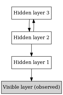
In machine learning, a deep belief network (DBN) is a generative graphical model, or alternatively a class of deep neural network, composed of multiple layers of latent variables ("hidden units"), with connections between the layers but not between units within each layer.
When trained on a set of examples without supervision, a DBN can learn to probabilistically reconstruct its inputs. The layers then act as feature detectors. After this learning step, a DBN can be further trained with supervision to perform classification.
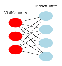
DBNs can be viewed as a composition of simple, unsupervised networks such as restricted Boltzmann machines (RBMs) or autoencoders, where each sub-network's hidden layer serves as the visible layer for the next. An RBM is an undirected, generative energy-based model with a "visible" input layer and a hidden layer and connections between but not within layers. This composition leads to a fast, layer-by-layer unsupervised training procedure, where contrastive divergence is applied to each sub-network in turn, starting from the "lowest" pair of layers (the lowest visible layer is a training set).
The observation that DBNs can be trained greedily, one layer at a time, led to one of the first effective deep learning algorithms. Overall, there are many attractive implementations and uses of DBNs in real-life applications and scenarios (e.g., electroencephalography, drug discovery).
Training
The training method for RBMs proposed by Geoffrey Hinton for use with training "Product of Experts" models is called contrastive divergence (CD). CD provides an approximation to the maximum likelihood method that would ideally be applied for learning the weights. In training a single RBM, weight updates are performed with gradient descent via the following equation:
where, is the probability of a visible vector, which is given by . is the partition function (used for normalizing) and is the energy function assigned to the state of the network. A lower energy indicates the network is in a more "desirable" configuration. The gradient has the simple form where represent averages with respect to distribution . The issue arises in sampling because this requires extended alternating Gibbs sampling. CD replaces this step by running alternating Gibbs sampling for steps (values of perform well). After steps, the data are sampled and that sample is used in place of . The CD procedure works as follows:
- Initialize the visible units to a training vector.
- Update the hidden units in parallel given the visible units: . is the sigmoid function and is the bias of .
- Update the visible units in parallel given the hidden units: . is the bias of . This is called the "reconstruction" step.
- Re-update the hidden units in parallel given the reconstructed visible units using the same equation as in step 2.
- Perform the weight update: .
Once an RBM is trained, another RBM is "stacked" atop it, taking its input from the final trained layer. The new visible layer is initialized to a training vector, and values for the units in the already-trained layers are assigned using the current weights and biases. The new RBM is then trained with the procedure above. This whole process is repeated until the desired stopping criterion is met.
Although the approximation of CD to maximum likelihood is crude (does not follow the gradient of any function), it is empirically effective.

See also
- Bayesian network
- Convolutional deep belief network
- Deep learning
- Energy based model
- Stacked Restricted Boltzmann Machine
References
- ^ Hinton G (2009). "Deep belief networks". Scholarpedia. 4 (5): 5947. Bibcode:2009SchpJ...4.5947H. doi:10.4249/scholarpedia.5947.
- ^ Hinton GE, Osindero S, Teh YW (July 2006). "A fast learning algorithm for deep belief nets" (PDF). Neural Computation. 18 (7): 1527–54. CiteSeerX 10.1.1.76.1541. doi:10.1162/neco.2006.18.7.1527. PMID 16764513. S2CID 2309950.
- Bengio Y, Lamblin P, Popovici D, Larochelle H (2007). Greedy Layer-Wise Training of Deep Networks (PDF). NIPS.
- Bengio, Y. (2009). "Learning Deep Architectures for AI" (PDF). Foundations and Trends in Machine Learning. 2: 1–127. CiteSeerX 10.1.1.701.9550. doi:10.1561/2200000006.
- Movahedi F, Coyle JL, Sejdic E (May 2018). "Deep Belief Networks for Electroencephalography: A Review of Recent Contributions and Future Outlooks". IEEE Journal of Biomedical and Health Informatics. 22 (3): 642–652. doi:10.1109/jbhi.2017.2727218. PMC 5967386. PMID 28715343.
- Ghasemi, Pérez-Sánchez; Mehri, Pérez-Garrido (2018). "Neural network and deep-learning algorithms used in QSAR studies: merits and drawbacks". Drug Discovery Today. 23 (10): 1784–1790. doi:10.1016/j.drudis.2018.06.016. PMID 29936244. S2CID 49418479.
- Ghasemi, Pérez-Sánchez; Mehri, fassihi (2016). "The Role of Different Sampling Methods in Improving Biological Activity Prediction Using Deep Belief Network". Journal of Computational Chemistry. 38 (10): 1–8. doi:10.1002/jcc.24671. PMID 27862046. S2CID 12077015.
- Gawehn E, Hiss JA, Schneider G (January 2016). "Deep Learning in Drug Discovery". Molecular Informatics. 35 (1): 3–14. doi:10.1002/minf.201501008. PMID 27491648. S2CID 10574953.
- Hinton GE (2002). "Training Product of Experts by Minimizing Contrastive Divergence" (PDF). Neural Computation. 14 (8): 1771–1800. CiteSeerX 10.1.1.35.8613. doi:10.1162/089976602760128018. PMID 12180402. S2CID 207596505.
- ^ Hinton GE (2010). "A Practical Guide to Training Restricted Boltzmann Machines". Tech. Rep. UTML TR 2010-003.
- Fischer A, Igel C (2014). "Training Restricted Boltzmann Machines: An Introduction" (PDF). Pattern Recognition. 47 (1): 25–39. Bibcode:2014PatRe..47...25F. CiteSeerX 10.1.1.716.8647. doi:10.1016/j.patcog.2013.05.025. Archived from the original (PDF) on 2015-06-10. Retrieved 2017-07-02.
- Bengio Y (2009). "Learning Deep Architectures for AI" (PDF). Foundations and Trends in Machine Learning. 2 (1): 1–127. CiteSeerX 10.1.1.701.9550. doi:10.1561/2200000006. Archived from the original (PDF) on 2016-03-04. Retrieved 2017-07-02.
External links
- Hinton, Geoffrey E. (2009-05-31). "Deep belief networks". Scholarpedia. 4 (5): 5947. Bibcode:2009SchpJ...4.5947H. doi:10.4249/scholarpedia.5947. ISSN 1941-6016.
- "Deep Belief Networks". Deep Learning Tutorials.
- "Deep Belief Network Example". Deeplearning4j Tutorials. Archived from the original on 2016-10-03. Retrieved 2015-02-22.

 is the probability of a visible vector, which is given by
  .
.  is the
  is the energy function assigned to the state of the network. A lower energy indicates the network is in a more "desirable" configuration. The gradient
  has the simple form
  where
where  represent averages with respect to distribution
  . The issue arises in sampling
  because this requires extended alternating
  steps (values of
  perform well). After
  .
.  is the
  is the bias of
  .
. .
.  is the bias of
  . This is called the "reconstruction" step.
 .
.