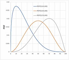
Probability density function Example density curves for the PERT probability distribution Example density curves for the PERT probability distribution | |||
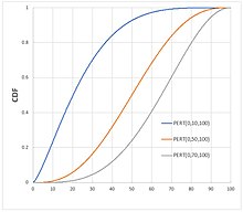
Cumulative distribution function Example cumulative distribution curves for the PERT probability distribution Example cumulative distribution curves for the PERT probability distribution | |||
| Parameters |
(real) (real) | ||
|---|---|---|---|
| Support | |||
|
where | |||
| CDF |
(the regularized incomplete beta function) with | ||
| Mean | |||
| Median |
| ||
| Mode | |||
| Variance | |||
| Skewness | |||
| Excess kurtosis | |||
In probability and statistics, the PERT distributions are a family of continuous probability distributions defined by the minimum (a), most likely (b) and maximum (c) values that a variable can take. It is a transformation of the four-parameter beta distribution with an additional assumption that its expected value is
The mean of the distribution is therefore defined as the weighted average of the minimum, most likely and maximum values that the variable may take, with four times the weight applied to the most likely value. This assumption about the mean was first proposed in Clark, 1962 for estimating the effect of uncertainty of task durations on the outcome of a project schedule being evaluated using the program evaluation and review technique, hence its name. The mathematics of the distribution resulted from the authors' desire to make the standard deviation equal to about 1/6 of the range. The PERT distribution is widely used in risk analysis to represent the uncertainty of the value of some quantity where one is relying on subjective estimates, because the three parameters defining the distribution are intuitive to the estimator. The PERT distribution is featured in most simulation software tools.
Comparison with the triangular distribution

The PERT distribution offers an alternative to using the triangular distribution which takes the same three parameters. The PERT distribution has a smoother shape than the triangular distribution. The triangular distribution has a mean equal to the average of the three parameters:
which (unlike PERT) places equal emphasis on the extreme values which are usually less-well known than the most likely value, and is therefore less reliable. The triangular distribution also has an angular shape that does not match the smoother shape that typifies subjective knowledge.
The modified-PERT distribution

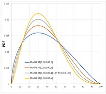
The PERT distribution assigns very small probability to extreme values, particularly to the extreme furthest away from the most likely value if the distribution is strongly skewed. The Modified PERT distribution was proposed to provide more control on how much probability is assigned to tail values of the distribution. The modified-PERT introduces a fourth parameter that controls the weight of the most likely value in the determination of the mean:
Typically, values of between 2 and 3.5 are used for and have the effect of flattening the density curve; the unmodified PERT would use . This is useful for highly skewed distributions where the distances and are of very different sizes.
The modified-PERT distribution has been implemented in several simulation packages and programming languages:
- ModelRisk – risk analysis add-in for Excel.
- Primavera risk analysis – project risk analysis simulation tool.
- Tamara – project risk analysis simulation tool.
- Wolfram Mathematica – mathematical symbolic computation program.
- R (programming language): mc2d package.
- Python (programming language): pertdist package.
References
- Clark CE (1962) The PERT model for the distribution of an activity. Operations Research 10, pp. 405406
- "PERT distribution". Vose Software. May 2, 2017. Retrieved July 16, 2017.
- Continuous Univariate Distributions - 2nd Ed (1995). Johnson K, Kotz S and Balakkrishnan N. (Section 25.4)
- Project Management Body of Knowledge: 5th Ed (2013). Project Management Institute Chapter 6
- Simulation Modeling and Analysis (2000). Law AM and Kelton WD. Section 6.11
- Business Risk and Simulation Modelling in Practice (2015). M Rees. Section 9.1.8
- Risk Analysis – a Quantitative Guide: 3rd Ed. (2008) Vose D
- Paulo Buchsbaum (June 9, 2012). "Modified Pert Simulation" (PDF). Greatsolutions.com.br. Archived from the original on December 23, 2018. Retrieved July 14, 2017.
- "Modified PERT distribution". Vose Software. May 2, 2017. Retrieved July 16, 2017.
- "Probability distributions used in Tamara". Vose Software. May 2, 2017. Retrieved July 16, 2017.
- "PERTDistribution—Wolfram Language Documentation". Reference.wolfram.com. Retrieved July 16, 2017.
- "Package 'mc2d'" (PDF). March 6, 2017. Retrieved December 16, 2020.
- "PertDist". December 6, 2020. Retrieved January 5, 2021.


 where
where


 that controls the weight of the most likely value in the determination of the mean:

 . This is useful for highly skewed distributions where the distances
  and
and  are of very different sizes.