In Vapnik–Chervonenkis theory, the Vapnik–Chervonenkis (VC) dimension is a measure of the size (capacity, complexity, expressive power, richness, or flexibility) of a class of sets. The notion can be extended to classes of binary functions. It is defined as the cardinality of the largest set of points that the algorithm can shatter, which means the algorithm can always learn a perfect classifier for any labeling of at least one configuration of those data points. It was originally defined by Vladimir Vapnik and Alexey Chervonenkis.
Informally, the capacity of a classification model is related to how complicated it can be. For example, consider the thresholding of a high-degree polynomial: if the polynomial evaluates above zero, that point is classified as positive, otherwise as negative. A high-degree polynomial can be wiggly, so it can fit a given set of training points well. But one can expect that the classifier will make errors on other points, because it is too wiggly. Such a polynomial has a high capacity. A much simpler alternative is to threshold a linear function. This function may not fit the training set well, because it has a low capacity. This notion of capacity is made rigorous below.
Definitions
VC dimension of a set-family
Let be a set family (a set of sets) and a set. Their intersection is defined as the following set family:
We say that a set is shattered by if contains all the subsets of , i.e.:
The VC dimension of is the cardinality of the largest set that is shattered by . If arbitrarily large sets can be shattered, the VC dimension is .
VC dimension of a classification model
A binary classification model with some parameter vector is said to shatter a set of generally positioned data points if, for every assignment of labels to those points, there exists a such that the model makes no errors when evaluating that set of data points.
The VC dimension of a model is the maximum number of points that can be arranged so that shatters them. More formally, it is the maximum cardinal such that there exists a generally positioned data point set of cardinality that can be shattered by .
Examples
- is a constant classifier (with no parameters); Its VC dimension is 0 since it cannot shatter even a single point. In general, the VC dimension of a finite classification model, which can return at most different classifiers, is at most (this is an upper bound on the VC dimension; the Sauer–Shelah lemma gives a lower bound on the dimension).
- is a single-parametric threshold classifier on real numbers; i.e., for a certain threshold , the classifier returns 1 if the input number is larger than and 0 otherwise. The VC dimension of is 1 because: (a) It can shatter a single point. For every point , a classifier labels it as 0 if and labels it as 1 if . (b) It cannot shatter all the sets with two points. For every set of two numbers, if the smaller is labeled 1, then the larger must also be labeled 1, so not all labelings are possible.
- is a single-parametric interval classifier on real numbers; i.e., for a certain parameter , the classifier returns 1 if the input number is in the interval and 0 otherwise. The VC dimension of is 2 because: (a) It can shatter some sets of two points. E.g., for every set , a classifier labels it as (0,0) if or if , as (1,0) if
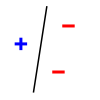
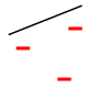
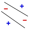
θ ∈ [ x − 2 , x ] {\displaystyle \theta \in } - is a straight line as a classification model on points in a two-dimensional plane (this is the model used by a perceptron). The line should separate positive data points from negative data points. There exist sets of 3 points that can indeed be shattered using this model (any 3 points that are not collinear can be shattered). However, no set of 4 points can be shattered: by Radon's theorem, any four points can be partitioned into two subsets with intersecting convex hulls, so it is not possible to separate one of these two subsets from the other. Thus, the VC dimension of this particular classifier is 3. It is important to remember that while one can choose any arrangement of points, the arrangement of those points cannot change when attempting to shatter for some label assignment. Note, only 3 of the 2 = 8 possible label assignments are shown for the three points.
- is a single-parametric sine classifier, i.e., for a certain parameter , the classifier returns 1 if the input number has and 0 otherwise. The VC dimension of is infinite, since it can shatter any finite subset of the set .

|

|

|

|
| 3 points shattered | 4 points impossible | ||
Uses
In statistical learning theory
The VC dimension can predict a probabilistic upper bound on the test error of a classification model. Vapnik proved that the probability of the test error (i.e., risk with 0–1 loss function) distancing from an upper bound (on data that is drawn i.i.d. from the same distribution as the training set) is given by:
where is the VC dimension of the classification model, , and is the size of the training set (restriction: this formula is valid when . When is larger, the test-error may be much higher than the training-error. This is due to overfitting).
The VC dimension also appears in sample-complexity bounds. A space of binary functions with VC dimension can be learned with:
samples, where is the learning error and is the failure probability. Thus, the sample-complexity is a linear function of the VC dimension of the hypothesis space.
In computational geometry
The VC dimension is one of the critical parameters in the size of ε-nets, which determines the complexity of approximation algorithms based on them; range sets without finite VC dimension may not have finite ε-nets at all.
Bounds
- The VC dimension of the dual set-family of is strictly less than , and this is best possible.
- The VC dimension of a finite set-family is at most . This is because by definition.
- Given a set-family , define as a set-family that contains all intersections of elements of . Then:
- Given a set-family and an element , define where denotes symmetric set difference. Then:
Examples of VC Classes
VC dimension of a finite projective plane
A finite projective plane of order n is a collection of n + n + 1 sets (called "lines") over n + n + 1 elements (called "points"), for which:
- Each line contains exactly n + 1 points.
- Each line intersects every other line in exactly one point.
- Each point is contained in exactly n + 1 lines.
- Each point is in exactly one line in common with every other point.
- At least four points do not lie in a common line.
The VC dimension of a finite projective plane is 2.
Proof: (a) For each pair of distinct points, there is one line that contains both of them, lines that contain only one of them, and lines that contain none of them, so every set of size 2 is shattered. (b) For any triple of three distinct points, if there is a line x that contain all three, then there is no line y that contains exactly two (since then x and y would intersect in two points, which is contrary to the definition of a projective plane). Hence, no set of size 3 is shattered.
VC dimension of a boosting classifier
Suppose we have a base class of simple classifiers, whose VC dimension is .
We can construct a more powerful classifier by combining several different classifiers from ; this technique is called boosting. Formally, given classifiers and a weight vector , we can define the following classifier:
The VC dimension of the set of all such classifiers (for all selections of classifiers from and a weight-vector from ), assuming , is at most:
VC dimension of a neural network
| This section needs additional citations for verification. Please help improve this article by adding citations to reliable sources in this section. Unsourced material may be challenged and removed. (May 2021) (Learn how and when to remove this message) |
A neural network is described by a directed acyclic graph G(V,E), where:
- V is the set of nodes. Each node is a simple computation cell.
- E is the set of edges, Each edge has a weight.
- The input to the network is represented by the sources of the graph – the nodes with no incoming edges.
- The output of the network is represented by the sinks of the graph – the nodes with no outgoing edges.
- Each intermediate node gets as input a weighted sum of the outputs of the nodes at its incoming edges, where the weights are the weights on the edges.
- Each intermediate node outputs a certain increasing function of its input, such as the sign function or the sigmoid function. This function is called the activation function.
The VC dimension of a neural network is bounded as follows:
- If the activation function is the sign function and the weights are general, then the VC dimension is at most .
- If the activation function is the sigmoid function and the weights are general, then the VC dimension is at least and at most .
- If the weights come from a finite family (e.g. the weights are real numbers that can be represented by at most 32 bits in a computer), then, for both activation functions, the VC dimension is at most .
Generalizations
The VC dimension is defined for spaces of binary functions (functions to {0,1}). Several generalizations have been suggested for spaces of non-binary functions.
- For multi-class functions (e.g., functions to {0,...,n-1}), the Natarajan dimension, and its generalization the DS dimension can be used.
- For real-valued functions (e.g., functions to a real interval, ), the Graph dimension or Pollard's pseudo-dimension can be used.
- The Rademacher complexity provides similar bounds to the VC, and can sometimes provide more insight than VC dimension calculations into such statistical methods such as those using kernels.
- The Memory Capacity (sometimes Memory Equivalent Capacity) gives a lower bound capacity, rather than an upper bound (see for example: Artificial neural network#Capacity) and therefore indicates the point of potential overfitting.
See also
- Growth function
- Sauer–Shelah lemma, a bound on the number of sets in a set system in terms of the VC dimension.
- Karpinski–Macintyre theorem, a bound on the VC dimension of general Pfaffian formulas.
Footnotes
- Vapnik, V. N.; Chervonenkis, A. Ya. (1971). "On the Uniform Convergence of Relative Frequencies of Events to Their Probabilities". Theory of Probability & Its Applications. 16 (2): 264. doi:10.1137/1116025. This is an English translation, by B. Seckler, of the Russian paper: "On the Uniform Convergence of Relative Frequencies of Events to Their Probabilities". Dokl. Akad. Nauk. 181 (4): 781. 1968. The translation was reproduced as: Vapnik, V. N.; Chervonenkis, A. Ya. (2015). "On the Uniform Convergence of Relative Frequencies of Events to Their Probabilities". Measures of Complexity. p. 11. doi:10.1007/978-3-319-21852-6_3. ISBN 978-3-319-21851-9.
- ^ Mohri, Mehryar; Rostamizadeh, Afshin; Talwalkar, Ameet (2012). Foundations of Machine Learning. US, Massachusetts: MIT Press. ISBN 9780262018258.
- Vapnik 2000.
- ^ Shalev-Shwartz, Shai; Ben-David, Shai (2014). Understanding Machine Learning – from Theory to Algorithms. Cambridge University Press. ISBN 9781107057135.
- Alon, N.; Haussler, D.; Welzl, E. (1987). "Partitioning and geometric embedding of range spaces of finite Vapnik-Chervonenkis dimension". Proceedings of the third annual symposium on Computational geometry – SCG '87. p. 331. doi:10.1145/41958.41994. ISBN 978-0897912310. S2CID 7394360.
- ^ Natarajan 1989.
- Brukhim 2022. sfn error: no target: CITEREFBrukhim2022 (help)
- Pollard 1984.
- Anthony & Bartlett 2009.
- Morgenstern & Roughgarden 2015.
- Karpinski & Macintyre 1997.
References
- Moore, Andrew. "VC dimension tutorial" (PDF).
- Vapnik, Vladimir (2000). The nature of statistical learning theory. Springer.
- Blumer, A.; Ehrenfeucht, A.; Haussler, D.; Warmuth, M. K. (1989). "Learnability and the Vapnik–Chervonenkis dimension" (PDF). Journal of the ACM. 36 (4): 929–865. doi:10.1145/76359.76371. S2CID 1138467.
- Burges, Christopher. "Tutorial on SVMs for Pattern Recognition" (PDF). Microsoft. (containing information also for VC dimension)
- Chazelle, Bernard. "The Discrepancy Method".
- Natarajan, B.K. (1989). "On Learning sets and functions". Machine Learning. 4: 67–97. doi:10.1007/BF00114804.
- Ben-David, Shai; Cesa-Bianchi, Nicolò; Long, Philip M. (1992). "Characterizations of learnability for classes of {O, …, n}-valued functions". Proceedings of the fifth annual workshop on Computational learning theory – COLT '92. p. 333. doi:10.1145/130385.130423. ISBN 089791497X.
- Brukhim, Nataly; Carmon, Daniel; Dinur, Irit; Moran, Shay; Yehudayoff, Amir (2022). "A Characterization of Multiclass Learnability". 2022 IEEE 63rd Annual Symposium on Foundations of Computer Science (FOCS). arXiv:2203.01550.
- Pollard, D. (1984). Convergence of Stochastic Processes. Springer. ISBN 9781461252542.
- Anthony, Martin; Bartlett, Peter L. (2009). Neural Network Learning: Theoretical Foundations. ISBN 9780521118620.
- Morgenstern, Jamie H.; Roughgarden, Tim (2015). On the Pseudo-Dimension of Nearly Optimal Auctions. NIPS. arXiv:1506.03684. Bibcode:2015arXiv150603684M.
- Karpinski, Marek; Macintyre, Angus (February 1997). "Polynomial Bounds for VC Dimension of Sigmoidal and General Pfaffian Neural Networks". Journal of Computer and System Sciences. 54 (1): 169–176. doi:10.1006/jcss.1997.1477.
 be a
be a  a set. Their intersection is defined as the following set family:

 contains all the subsets of
 of
of  .
.
 with some parameter vector
  is said to
  if, for every assignment of labels to those points, there exists a
  different classifiers, is at most
  (this is an upper bound on the VC dimension; the
  returns 1 if the input number is larger than
  , a classifier
  and labels it as 1 if
  . (b) It cannot shatter all the sets with two points. For every set of two numbers, if the smaller is labeled 1, then the larger must also be labeled 1, so not all labelings are possible.
 and 0 otherwise. The VC dimension of
  , a classifier
  or if
or if  , as (1,0) if
 , and as (0,1) if
 ![{\displaystyle \theta \in (x,x+2]}](https://wikimedia.org/api/rest_v1/media/math/render/svg/b4adcdf37171b523669f5352c245d8de775ab92f) . (b) It cannot shatter any set of three points. For every set of three numbers, if the smallest and the largest are labeled 1, then the middle one must also be labeled 1, so not all labelings are possible.
. (b) It cannot shatter any set of three points. For every set of three numbers, if the smallest and the largest are labeled 1, then the middle one must also be labeled 1, so not all labelings are possible. and 0 otherwise. The VC dimension of
  .
.
 , and
, and  is the size of the training set (restriction: this formula is valid when
  . When
 is the learning error and
  is the failure probability. Thus, the sample-complexity is a linear function of the VC dimension of the hypothesis space.
 is strictly less than
  , and this is best possible.
 . This is because
  by definition.
 as a set-family that contains all intersections of
  elements of
 , define
  where
where  denotes
 of simple classifiers, whose VC dimension is
  classifiers
  and a weight vector
  , we can define the following classifier:

 ), assuming
  , is at most:

 .
. and at most
  .
. .
.